Orthogonal instrumental variables

What is it?

Orthogonal instrumental variables is a suite of methods to estimate heterogeneous treatment effects with arbitrary machine learning methods in the presence of unobserved confounders with the aid of a valid instrument. We develop a statistical learning approach to the estimation of heterogeneous effects, reducing the problem to the minimization of an appropriate loss function that depends on a set of auxiliary models (each corresponding to a separate prediction task). The reduction enables the use of all recent Machine Learning models (e.g. random forest, boosting, neural nets). We show that the estimated effect model is robust to estimation errors in the auxiliary models, by showing that the loss satisfies a Neyman orthogonality criterion. Our approach can be used to estimate projections of the true effect model on simpler hypothesis spaces. When these spaces are parametric, then the parameter estimates are asymptotically normal, which enables construction of confidence intervals. For a more detailed overview of these methods, see e.g. [Syrgkanis2019].

What are the relevant estimator classes?

This section describes the methodology implemented in the classes OrthoIV, DMLIV, NonParamDMLIV, LinearDRIV, SparseLinearDRIV, ForestDRIV, IntentToTreatDRIV, LinearIntentToTreatDRIV. Click on each of these links for detailed module documentation and input parameters of each class.

When should you use it?

Suppose you have observational (or experimental from an A/B test) historical data, where some treatment(s)/intervention(s)/action(s) \(T\) were chosen and some outcome(s) \(Y\) were observed. However, not all of the variables \(W\) that could have potentially gone into the choice of \(T\), and simultaneously could have had a direct effect on the outcome \(Y\) (aka controls or confounders) are recorded in the dataset. At the same time if you could observe a variable \(Z\) which will have a direct effect on treatment and an indirect effect on outcome which only goes through the treatment, we could use classes mentioned above to learn the heterogeneous treatment effect on high dimensional dataset. In other words, we learn the effect of the treatment on the outcome as a function of a set of observable characteristics \(X\).

In particular, these methods are especially useful in A/B tests with an intent-to-treat structure, where the experimenter randomizes over which user will receive a recommendation to take an action, and we are interested in the effect of the downstream action.

For instance call:

from econml.iv.dr import LinearIntentToTreatDRIV
est = LinearIntentToTreatDRIV()
est.fit(y, T, Z=Z, X=X, W=X)
est.effect(X)

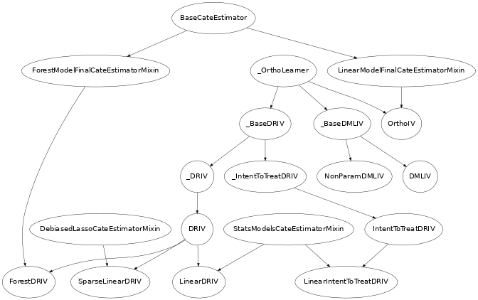
Class Hierarchy Structure

In this library we implement variants of several of the approaches mentioned in the last section. The hierarchy structure of the implemented CATE estimators is as follows.

Usage Examples

For more extensive examples check out the following notebooks: OrthoIV and DRIV Examples Jupyter Notebook.